Shift Change on the Factory Floor

Picture a line of bots gliding past pallet racks as the buzzer hits shift change, and one unit hesitates at a blind turn. Your heart hears it before your head does. The amr controller is doing its best, but the beat is off by a few milliseconds. Last quarter, your logs showed 11% of micro-stops came from command delays and jitter. That’s not a melody you want to repeat. So ask yourself: is this a sensor quirk or a sign the control brain has outgrown its stage?

We speak about machines like instruments because timing is everything—tempo, dynamics, feel. That’s why small delays cascade into big costs. A 120 ms rise in command latency can turn a clean merge into a stall. Multiply that by a fleet, and you hear the echo across your KPIs. And yet, we often tweak around the edges, hoping for a better chorus from the same old score (been there, done that). What happens when another tune-up won’t fix the groove? Let’s step into the comparison that matters next.

The Quiet Friction Inside Your Control Stack

Why do legacy loops drift?

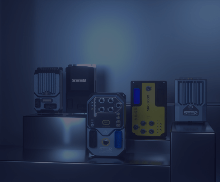
Here’s the straight read: the industrial robot control system in many plants was built for slower rhythms and simpler maps. Legacy stacks push motion commands through layers that were never tuned for tight, mixed-traffic spaces with dynamic loads. Every hop adds jitter. CAN bus bursts pile up. Sensor fusion waits a hair too long for that last Lidar frame. Then the motion planner compensates, and your path looks fine on paper but ragged in reality—funny how that works, right?

Most teams feel the symptom, not the source. You see a stall, so you add a patch. Another watchdog. A stiffer PID loop. Maybe higher current on actuator drivers via the power converters. But hidden pain points remain: non-deterministic queues, a real-time OS pushed to its margin, and fieldbus bandwidth that cracks during peak traffic. Look, it’s simpler than you think: if edge computing nodes can’t pre-resolve the heavy math—collision checks, SLAM updates—before the control window closes, the robot starts to “sing late.” That late note costs you meters per hour, and sometimes safety margins too.

From Legacy Loops to Learning Controllers: What Changes and Why

What’s Next

Let’s move to a forward-looking lens—comparative and practical. Newer controller designs shift from poll-heavy, layer-stacked paths to event-driven, time-aware networks. Think deterministic Ethernet with TSN, priority lanes for motion-critical packets, and QoS that favors the brake command over the debug stream. The heart of the industrial robot control system becomes simpler and faster: fewer hops, smarter buffering, and model predictive control that anticipates load and traction changes one beat ahead. It’s not magic; it’s architecture.

Now compare outcomes on the floor. A legacy rack might hold 90 ms median loop time—fine until traffic spikes and you see 220 ms tails. A next-gen stack keeps tails tight, under 120 ms, even when SLAM updates run hot. Why? Work moves closer to the edge. Maps compress. Sensor traces are pre-filtered before they hit the motion planner. And the controller prioritizes intent over noise—brake, steer, and accelerate get guaranteed slots, while logs trickle later. Small change, big feel. Your fleet flows, not stutters.

There’s a people side too. Teams swap from reactive tuning to proactive planning. You measure per-route latency, not just average loop time. You watch energy per meter and thermal headroom at the drive stage. You run “what-if” loads in a sandbox copy of your industrial robot control system before the night shift. And yes, the learning curve is real—but the return is tangible, month after month.

Advisory close: when choosing an upgrade path, track three metrics that matter. One, deterministic latency under load (P95 and P99, not just the median). Two, mean recovery time from sensor-drop or comms fault (from event to stable state). Three, energy per meter moved at rated payload (Wh/m) across your key routes. Compare these across candidates, same maps, same traffic—apples to apples—and your choice will be clear. For deeper technical references and tools, see resources from SEER Robotics—and build your next set to play in time.